|
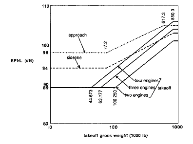
Реферат: Tupolev 154M noise asesment (Анализ шумовых характеристик самолёта Ту-154М)The new rules have been applied only to subsonic transports, because no new supersonic commercial aircraft have been developed since its promulgation. 5.1 Noise LimitsAs mentioned above, all turbofan-powered transport aircraft must comply at certification with EPNL limits for the three measuring stations as shown in Fig. 5.1. The limits depend on the gross weight of the aircraft at take-off and number of engines, as shown in Fig. 5.2. The rule is the same for all engine numbers on approach and on the sideline because the distance from the aircraft to the measuring point is fixed on approach by the angle of the approach path (normally 3 deg) and on the sideline by the distance of the measuring station from the runway centerline.
Figure 5.2 Noise limits imposed by ICAO Annex 16 for certification of aircraft. On take-off, however, aircraft with fewer engines climb out faster, so they are higher above the measuring point. Here the “reasonable and economically practicable” principle comes into dictate that three-engine and two-engine aircraft have lower noise levels at the take-off noise station than four-engine aircraft. There is some flexibility in the rule, in that the noise levels can be exceeded by up to 2 EPNdB at any station provided the sum of the exceedances is not over 3 ENPdB and that the exceedances are completely offset by reductions at other measuring stations. 6 Noise Level Calculations6.1 Tupolev 154M DescriptionFor most airlines in the CIS, the Tupolev Tu-154 is nowadays the workhorse on domestic and international routes.
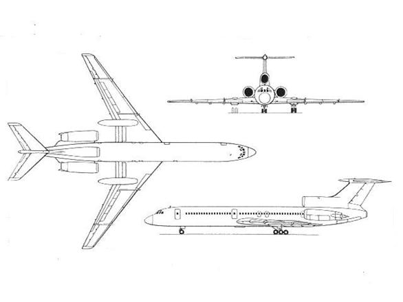
Figure 6.1 Tupolev 154M main look It was produced in two main vesions: The earlier production models have been designated Tupolev -154, Tupolev -154A, Tupolev -154B, Tupolev -154B-1 and Tupolev -154B-2, while the later version has been called Tupolev -154M. Overall, close to 1'000 Tupolev -154s were built up to day, of which a large portion is still operated. Table 6.1 Tupolev 154M main characteristics
The Tu-154 was developed to replace the turbojet powered Tupolev Tu-104, plus the Antonov - 10 and Ilyushin - 18 turboprops. Design criteria in replacing these three relatively diverse aircraft included the ability to operate from gravel or packed earth airfields, the need to fly at high altitudes 'above most Soviet Union air traffic, and good field performance. In meeting these aims the initial Tupolev -154 design featured three Kuznetsov (now KKBM) NK-8 turbofans, triple bogey main undercarriage units which retract into wing pods and a rear engine T-tail configuration. The Tupolev -154's first flight occurred on October 4 1968. Regular commercial service began in February 1972. Three Kuznetsov powered variants of the Tupolev -154 were built, the initial Tupolev -154, the improved Tupolev -154A with more powerful engines and a higher max take-off weight and the Tupolev -154B with a further increased max take-off weight. Tupolev -154S is a freighter version of the Tupolev -154B. Current production is of the Tupolev -154M, which first flew in 1982. The major change introduced on the M was the far more economical, quieter and reliable Solovyev (now Aviadvigatel) turbofans. The Tupolev - 154M2 is a proposed twin variant powered by two Perm PS90A turbofans. 6.2 Noise CalculaionsNoise level at control points is calculated using the Noise-Power-Distance (NPD) relationship. In practice NPD-relationship is used in the parabolic shape:
where coefficients А, В, С are different for different aircraft types and engine modes. For Tupolev-154M the coefficients А, В, С are shown in the table 6.2 in respect to Tupolev-154. Table 6.2 Noise-Power-Distance coefficients of similar aircraft.
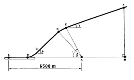
6.2.1 Take-off Noise CalculationThe aircraft begins the take-off roll at point A (Fig. 6.2), lifts off at point B, and initiates the first constant climb at point C at an angle β. The noise abatement thrust cutback is started at point D and completed at point E where the second constant climb is defined by the angle γ (usually expressed in terms of the gradient in percent). The end of the noise certification take-off flight path is represented by aircraft position F whose vertical projection on the flight track (extended centerline of the runway) is point M. The position of the aircraft must be recorded for the entire interval during which the measured aircraft noise level is within 10 dB of PNLTM. Position K is the take-off noise measuring station whose distance AK is specified as 6500 meters.
Figure 6.2 Take-off and climb path The take-off profile is defined by five parameters -- (A) AB, the length of take-off roll; (B) β the first constant climb angle; (C) γ, the second constant climb angle; and (D) δ, and e, the thrust cutback angles. These five parameters are functions of the aircraft performance and weight, and the atmospheric conditions of temperature, pressure, and wind velocity and direction. Under reference atmospheric conditions and with maximum take-off weight, the gradient of the second constant climb angle (γ) may not be less than 4 percent. However, the actual gradient will depend upon atmospheric conditions, assuming maximum take-off weight and the parameters characterizing engine performance are constant (rpm, or any other parameter used by the pilot). In operational conditions the climb is performed without the cutback stage, and the aircraft flies over the control point at a lower altitude, which leads to higher noise levels.
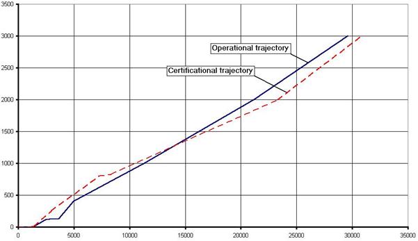
Figure 6.3 Comparison between operational and certification trajectories The climb path for Tupolev 154M was calculated using the following equation
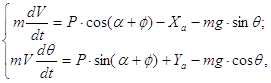
where: m is aircraft mass; P is thrust; a is the angle of attack, j is the angle of engine installation; q is climb angle which is equal to b or g, depending on the climb stage.
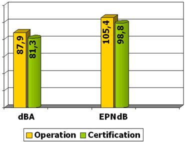
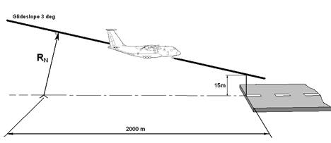
Figure 6.4 Comparison between noise levels under different flight paths 6.2.2 Approach Noise CalculationThe approaches must be conducted with a steady glide angle of 3°±0.5° and must be continued to a normal touchdown with no airframe configuration change. Thus the distance from the control point to the glideslope RN remains constant and is equal to 119.7 m. |
||||||||||||||||||||||||||||||||||||||||||||||||||||||||||||||||||||||||||||||||||||||||||||||||||||||||||||||||||||||||||||||||||||||||||||||||||||||||||||||||||||||||||||||||||||||||||||||||||||||||||||||||||||||||||||||||
| Weight, % MLW | MLW | 95% | 90% | 85% | 80% |
| Weight, kg | 80000 | 76000 | 72000 | 68000 | 68000 |
| Vapp, m/s | 74,8 | 72,91 | 70,964 | 68,965 | 66,91 |
| Thrust, kg | 8445,63 | 8024,67 | 7601,88 | 7179,66 | 6758,58 |
|
LA, dBA |
96,74 | 96,05 | 95,35 | 94,66 | 93,97 |
| EPNL, EPNdB | 112,17 | 111,32 | 110,48 | 109,64 | 108,79 |
| ∆LA, dBA | 0 | 0,69 | 0,7 | 0,69 | 0,69 |
| ∆EPNL, EPNdB | 0 | 0,85 | 0,84 | 0,84 | 0,85 |
| SQRT (Wing Load) | 21,082 | 20,548 | 20 | 19,437 | 18,856 |
| Thrust To Weight rt. | 0,10557 | 0,105588 | 0,105582 | 0,105583 | 0,105603 |
Tupolev 154M has the same aerodynamics as Tupolev 154, thus the necessary thrust for both of them during approach is almost the same. Tupolev 154M has more powerful engines and it can carry more payload. Its maximum landing weight is 2 tons greater than that one of 154. Noise parameters are different for these aircraft (table 6.2), and the calculated noise levels slightly differ as well.
Methods for suppressing jet noise have exploited the characteristics of the jet itself and those of the human observer. For a given total noise power, the human impact is less if the frequency is very high, as the ear is less sensitive at high frequencies. A shift to high frequency can be achieved by replacing one large nozzle with many small ones. This was one basis for the early turbojet engine suppressors. Reduction of the jet velocity can have a powerful effect since P is proportional to the jet velocity raised to a power varying from 8 to 3, depending on the magnitude of uc. The multiple small nozzles reduced the mean jet velocity somewhat by promoting entrainment of the surrounding air into the jet. Some attempts have been made to augment this effect by enclosing the multinozzle in a shroud, so that the ambient air is drawn into the shroud.
Certainly the most effective of jet noise suppressors has been the turbofan engine, which in effect distributes the power of the exhaust jet over a larger airflow, thus reducing the mean jet velocity.
In judging the overall usefulness of any jet noise reduction system, several factors must be considered in addition to the amount of noise reduction. Among these factors are loss of thrust, addition of weight, and increased fuel consumption.
A number of noise-suppression schemes have been studied, mainly for turbofan engines of one sort or another. These include inverted-temperature-profile nozzles, in which a hot outer flow surrounds a cooler core flow, and mixer-ejector nozzles. In the first of these, the effect is to reduce the overall noise level from that which would be generated if the hot outer jets are subsonic with respect to the outer hot gas. This idea can be implemented either with a duct burner on a conventional turbofan or with a nozzle that interchanges the core and duct flows, carrying the latter to the inside and the former to the outside. In the mixer-ejector nozzle, the idea is to reduce the mean jet velocity by ingesting additional airflow through a combination of the ejector nozzles and the chute-type mixer. Fairly high mass flow ratios can be attained with such arrangements, at the expense of considerable weight.
The most promising solution, however, is some form of “variable cycle” engine that operates with a higher bypass ratio on take-off and in subsonic flight than at the supersonic cruise condition. This can be achieved to some degree with multi-spool engines by varying the speed of some of the spools to change their mass flow, and at the same time manipulating throttle areas. Another approach is to use a tandem-parallel compressor arrangement, where two compressors operate in parallel at take-off and subsonically, and in series at a supersonic conditions.
It is self evident that the most desirable way to reduce engine noise would be to eliminate noise generation by changing the engine design. The current state of the art, however, will not provide levels low enough to satisfy expected requirements; thus, it is necessary to attenuate the noise that is generated.
Fan noise radiated from the engine inlet and fan discharge (Fig. 7.1) of current fan jet airplanes during landing makes the largest contribution to perceived noise.
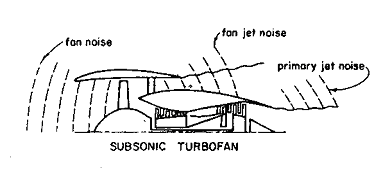
Figure 7.1 Schematic illustration of noise sources from turbofan engines
Figure 7.2. shows a typical farfield SPL noise spectrum generated by a turbofan engine at a landing-approach power setting. Below 800 Hz, the spectrum is controlled by noise from the primary jet exhaust. The spectrum between 800 and 10000 Hz contains several discrete frequency components in particular that need to be attenuated by the linings in the inlet and the fan duct before they are radiated to the farfield.
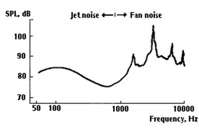
Figure 7.2 Engine-noise spectrum
The objective in applying acoustic treatment is to reduce the SPL at the characteristic discrete frequencies associated with the fan blade passage frequency and its associated harmonics. Noise reductions at these frequencies would alleviate the undesirable fan whine and would reduce the perceived noise levels.
A promising approach to the problem has been the development of a tuned-absorber noise-suppression system that can be incorporated into the inlet and exhaust ducts of turbofan engines. An acoustical system of this type requires that the internal aerodynamic surfaces of the ducts be replaced by sheets of porous materials, which are backed by acoustical cavities. Simply, these systems function as a series of dead-end labyrinths, which are designed to trap sound waves of a specific wavelength. The frequencies for which these absorbers are tuned is a function of the porosity of flow resistance of the porous facing sheets and of the depth or volume of the acoustical cavities. The cavity is divided into compartments by means of an open cellular structure, such as honeycomb cells, to provide an essentially locally reacting impedance (Fig. 7.3). This is done to provide an acoustic impedance almost independent of the angle of incidence of the sound waves impinging on the lining.
The perforated-plate-and-honeycomb combination is similar to an array of Helmholtz resonators; the pressure in the cavity acts as a spring upon which the flow through the orifice oscillates in response to pressure fluctuations outside the orifice.
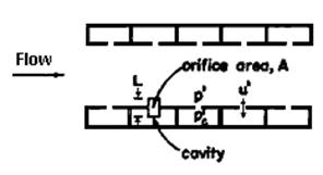
Figure 7.2 Schematic of acoustic damping cavities in an angine duct. The size of the resonators
is exaggerated relative to the duct diameter.
The attenuation spectrum of this lining is that of a sharply tuned resonator effective over a narrow frequency range when used in an environment with low airflow velocity or low SPL. This concept, however, can also provide a broader bandwidth of attenuation in a very high noise-level environment where the particle velocity through the perforations is high, or by the addition of a fine wire screen that provides the acoustic resistance needed to dissipate acoustic energy in low particle-velocity or sound-pressure environments. The addition of the wire screen does, however, complicate manufacture and adds weight to such an extent that other concepts are usually more attractive.
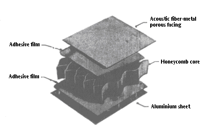
Figure 7.3 Acoustical lining structure.
Although the resistive-resonator lining is a frequency-tuned device absorbing sound in a selected frequency range, a suitable combination of material characteristics and lining geometry will yield substantial attenuation over a frequency range wide enough to encompass the discrete components and the major harmonics of most fan noise.
First we have to determine the blade passage frequency:
![]() ,
,
where z is number of blades, n is RPM.
Blade passage frequencies for different engine modes are given in table 7.1
Next we determine the
second fan blade passage harmonic frequency, which is two times greater than
the first one: ![]() .
.
Table 7.1 Fan blade passage frequencies for different engine modes.
| Take-off | Nominal | 88%Nom | 70%Nom | 60%Nom | 53%Nom | Idle | ||||||||
| RPM | 10425 | 10055 | 9878 | 9513 | 9315 | 8837 | 4000 | |||||||
|
1st harmonic freq., Hz |
|
|
|
|
|
|
|
|||||||
|
2nd harmonic freq., Hz |
|
|
|
|
|
|
|
Using experimental data, we determine lining and cell geometry:
For the first harmonic, parameters will be:
· Distance between linings 28.5 cm;
· Lining length 45 cm;
· Lining depth 2.5 cm;
· Cell length 2 cm..
For the second harmonic, parameters will be the following:
· Distance between linings 4.5 cm;
· Lining length 5 cm;
· Lining depth 2.5 cm;
· Cell length 0.4 cm.
Figure 7.4 shows the placement of the lining in engine nacelle.
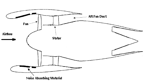
Figure 7.4 Lining placement in the nacelle.
Страницы: 1, 2
 |
||
| НОВОСТИ |  |
|
|
||
| ВХОД | |
|
|
|||||
Рефераты бесплатно, реферат бесплатно, курсовые работы, реферат, доклады, рефераты, рефераты скачать, рефераты на тему, сочинения, курсовые, дипломы, научные работы и многое другое. |
||
При использовании материалов - ссылка на сайт обязательна. |
||

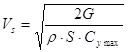 ,
,
 is drag and q is approach path angle
which is equal to 3 degrees.
is drag and q is approach path angle
which is equal to 3 degrees.